Excel INDEX MATCH with multiple criteria - formula examples

by Svetlana Cheusheva , updated on March 14, 2023

The tutorial shows how to lookup with multiple criteria in Excel using INDEX and MATCH and a few other ways.

Although Microsoft Excel provides special functions for vertical and horizontal lookup, expert users normally replace them with INDEX MATCH, which is superior to VLOOKUP and HLOOKUP in many ways. Among other things, it can look up two or more criteria in columns and rows. This tutorial explains the syntax and inner mechanics in full detail so that you can easily adjust the formula for your particular needs. To make the examples easier to follow, you are welcome to download our sample workbook.

Excel INDEX MATCH with multiple criteria

When working with large databases, you may sometimes find yourself in a situation when you need to find something but don't have a unique identifier for the search. In this case, lookup with several conditions is the only solution.

To look up a value based on multiple criteria in separate columns, use this generic formula:

• Return_range is the range from which to return a value.
• Criteria1, criteria2, … are the conditions to be met.
• Range1, range2, … are the ranges on which the corresponding criteria should be tested.

Important note! This is an array formula and it must be completed with Ctrl + Shift + Enter . This will enclose your formula in , which is a visual sign of an array formula in Excel. Do not try typing the braces manually, that won't work!

The formula is an advanced version of the iconic INDEX MATCH that returns a match based on a single criterion. To evaluate multiple criteria, we use the multiplication operation that works as the AND operator in array formulas. Below, you will find a real-life example and the detailed explanation of the logic.

Tip. In Excel 365 and 2021, you can use XLOOKUP formula with multiple criteria.

INDEX MATCH with several criteria - formula example

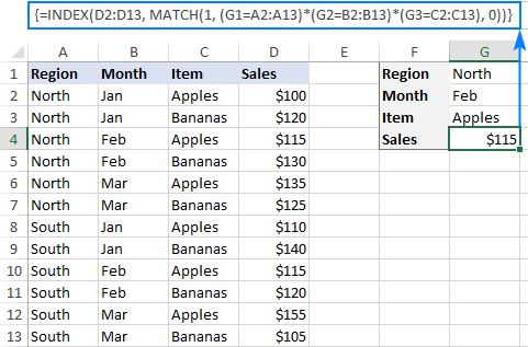
For this example, we will be using a table in the so-called "flat-file" format with each separate criteria combination (region-month-item in our case) on its own row. Our goal is to retrieve the sales figure for a certain item in a specific region and month.

With the source data and criteria in the following cells:

• Return_range (sales) - D2:D13
• Criteria1 (target region) - G1
• Criteria2 (target month) - G2
• Criteria3 (target item) - G3
• Range1 (regions) - A2:A13
• Range2 (months) - B2:B13
• Range3 (items) - C2:C13

The formula takes the following shape:

=INDEX(D2:D13, MATCH(1, (G1=A2:A13) * (G2=B2:B13) * (G3=C2:C13), 0))

Enter the formula, say in G4, complete it by pressing Ctrl + Shift + Enter and you will get the following result:

How this formula works

The trickiest part is the MATCH function, so let's figure it out first:

MATCH(1, (G1=A2:A13) * (G2=B2:B13) * (G3=C2:C13), 0))

As you may remember, MATCH(lookup_value, lookup_array, [match_type]) searches for the lookup value in the lookup array and returns the relative position of that value in the array.

In our formula, the arguments are as follows:

• Lookup_value: 1
• Lookup_array: (G1=A2:A13) * (G2=B2:B13) * (G3=C2:C13)
• Match_type: 0

The 1 st argument is crystal clear - the function searches for the number 1. The 3 rd argument set to 0 means an "exact match", i.e. the formula returns the first found value that is exactly equal to the lookup value.

The question is - why do we search for "1"? To get the answer, let's have a closer look at the lookup array where we compare each criterion against the corresponding range: the target region in G1 against all regions (A2:A13), the target month in G2 against all months (B2:B13) and the target item in G3 against all items (C2:C13). An intermediate result is 3 arrays of TRUE and FALSE where TRUE represents values that meet the tested condition. To visualize this, you can select the individual expressions in the formula and press the F9 key to see what each expression evaluates to:

The multiplication operation transforms the TRUE and FALSE values into 1's and 0's, respectively:

And because multiplying by 0 always gives 0, the resulting array has 1's only in the rows that meet all the criteria:

The above array goes to the lookup_array argument of MATCH. With lookup_value of 1, the function returns the relative position of the row for which all the criteria are TRUE (row 3 in our case). If there are several 1's in the array, the position of the first one is returned.

The number returned by MATCH goes directly to the row_num argument of the INDEX(array, row_num, [column_num]) function:

And it yields a result of $115, which is the 3 rd value in the D2:D13 array.

Non-array INDEX MATCH formula with multiple criteria

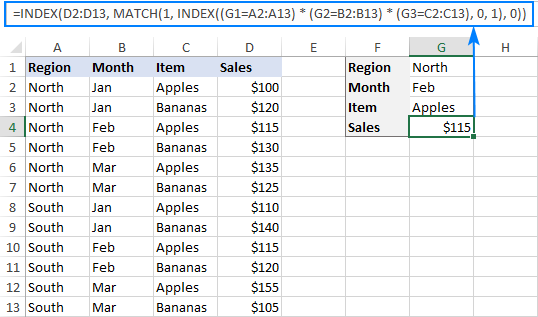
The array formula discussed in the previous example works nice for experienced users. But if you are building a formula for someone else and that someone does not know array functions, they may inadvertently break it. For example, a user may click your formula to examine it, and then press Enter instead of Ctrl + Shift + Enter . In such cases, it would be wise to avoid arrays and use a regular formula that is more bulletproof:

For our sample dataset, the formula goes as follows:

=INDEX(D2:D13, MATCH(1, INDEX((G1=A2:A13) * (G2=B2:B13) * (G3=C2:C13), 0, 1), 0))

How this formula works

As the INDEX function can process arrays natively, we add another INDEX to handle the array of 1's and 0's that is created by multiplying two or more TRUE/FALSE arrays. The second INDEX is configured with 0 row_num argument for the formula to return the entire column array rather than a single value. Since it's a one-column array anyway, we can safely supply 1 for column_num:

This array is passed to the MATCH function:

MATCH finds the row number for which all the criteria are TRUE (more precisely, the the relative position of that row in the specified array) and passes that number to the row_num argument of the first INDEX:

INDEX MATCH with multiple criteria in rows and columns

This example shows how to perform lookup by testing two or more criteria in rows and columns. In fact, it's a more complex case of the so-called "matrix lookup" or "two-way lookup" with more than one header row.

Here's the generic INDEX MATCH formula with multiple criteria in rows and columns:

<=INDEX(table_array, MATCH(vlookup_value, lookup_column, 0), MATCH(hlookup_value1 & hlookup_value2, lookup_row1 & lookup_row2, 0))>

Table_array - the map or area to search within, i.e. all data values excluding column and rows headers.

Vlookup_value - the value you are looking for vertically in a column.

Lookup_column - the column range to search in, usually the row headers.

Hlookup_value1, hlookup_value2, … - the values you are looking for horizontally in rows.

Lookup_row1, lookup_row2, … - the row ranges to search in, usually the column headers.

Important note! For the formula to work correctly, it must be entered as an array formula with Ctrl + Shift + Enter .

It is a variation of the classic two-way lookup formula that searches for a value at the intersection of a certain row and column. The difference is that you concatenate several hlookup values and ranges to evaluate multiple column headers. To better understand the logic, please consider the following example.

Matrix lookup with multiple criteria - formula example

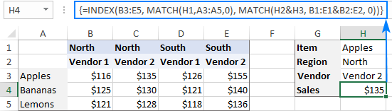
In the sample table below, we'll be searching for a value based on the row headers (Items) and 2 column headers (Regions and Vendors). To make the formula easier to build, let's first define all the criteria and ranges:

• Table_array - B3:E4
• Vlookup_value (target item) - H1
• Lookup_column (Row headers: items) - A3:A4
• Hlookup_value1 (target region) - H2
• Hlookup_value2 (target vendor) - H3
• Lookup_row1 (Column headers 1: regions) - B1:E1
• Lookup_row2 (Column headers 2: vendors) - B2:E2

And now, supply the arguments into the generic formula explained above, and you will get this result:

=INDEX(B3:E5, MATCH(H1,A3:A5,0), MATCH(H2&H3,B1:E1&B2:E2,0))

Remember to complete the formula by pressing the Ctrl + Shift + Enter shortcut, and your matrix lookup with multiple criteria will be done successfully:

How this formula works

As we are searching vertically and horizontally, we need to supply both the row and column numbers for the INDEX(array, row_num, column_num) function.

Row_num is delivered by MATCH(H1, A3:A5, 0) that compares the target item (Apples) in H1 against the row headers in A3:A5. This gives a result of 1 because "Apples" is the 1st item in the specified range.

Column_num is worked out by concatenating 2 lookup values and 2 lookup arrays: MATCH(H2&H3, B1:E1&B2:E2, 0))

The key factor for success is that the lookup values should match the column headers exactly and be concatenated in the same order. To visualize this, select the first two arguments in the MATCH formula, press F9 , and you will see what each argument evaluates to:

As "NorthVendor 2" is the second element in the array, the function returns 2.

At this point, our lengthy two-dimensional INDEX MATCH formula transforms into this simple one:

And returns a value at the intersection of the 1st row and 2nd column in the range B3:E5, which is the value in the cell C3.

That's how to look up multiple criteria in Excel. I thank you for reading and hope to see you on our blog next week!

Practice workbook for download

How to look up several conditions in Excel

• VLOOKUP with multiple criteria – requires adding a helper column to your table. That's not a very elegant solution, but you may want to know all available options.
• XLOOKUP with multiple criteria – the recent addition to the family of Excel's lookup and reference functions handles arrays by design. Meaning, it works as a regular formula, not an array formula!
• Lookup multiple conditions and return multiple results - combine 5 different functions in a single formula to evaluate several criteria and return all matches either in a column or row.
• INDEX MATCH MATCH formula in Excel – a few different ways to perform two dimensional lookup in Excel.
• Merge Tables Wizard - visual way to Vlookup in Excel with one or more criteria.
• Excel XLOOKUP vs INDEX MATCH - See how to use the new XLOOKUP function instead of the longstanding INDEX MATCH combo.

Table of contents

283 comments

Hi! Thank you very much, this has been very useful. Can I please have some advice? Please excuse my lack of technical terms, I'm new to Excel. I would like to input a figure (commodity code) into cell D2 and have the formula search for all exact matches in column B (commodity codes for each product on purchase order) once the formula has located each cell containing the commodity code in column B it will add up all matching data in column A and output the total figure into C2? FOR EXAMPLE: A B C D
Net Weight Commodity Code Total Net Weight for Specific Commodity Code Specific Commodity Code
0.36 4202990090 12.6 4202990090
7.60 4202990090
0.10 9004909000
0.08 9004909000
4.20 4202990090 Apologies if I haven't explained my question very well.
If you can please help me with my query I will be very grateful ! Thanks
Connor

Hi! You can calculate sum of values by condition using SUMIF function. If you are calculating the sum of multiple conditions, use this guide: Excel SUMIFS and SUMIF with multiple criteria – formula examples.
If I understand your task correctly, the formula might look something like this: =SUMIF(B2:B10,D2,A2:A10)

I'm creating a team schedule from logged future appointments across multiple people and I want to return the appointment name next to the relevant time slots that it spans over. =IFERROR(INDEX('CRM Schedule'!B:B,MATCH(1,INDEX((Schedule!D7>='CRM Schedule'!L:L)*(Schedule!D7 Alexander Trifuntov (Ablebits Team) says:
2024-06-07 at 1:32 pm

Hi! To determine a partial matching of a name in E2 and a record in the CRM Schedule Sheet, use these guidelines: How to find substring in Excel.
Replace formula (Schedule!$E$2='CRM Schedule'!J:J) with ISNUMBER(SEARCH(Schedule!$E$2,'CRM Schedule'!J:J)). This will identify a partial match between the values in E2 and column J.
I can't check your entire formula as I don't have your data.

Just wanted to say thanks for this excellent article. Explained a fairly complex idea in an easy to understand way and solved a problem I had trying to extract some data out of an Excel data table that had been causing me some problems . Cracked it thanks to this article.

How to search, compare and match a value from a cell in one template with an instance of a value (not a full cell match) in a row from a second template and return a value from different columns from the second template

Hi! To use a partial match of text strings as searching criteria, use the SEARCH function as described in this guide: How to find substring in Excel. For example: =INDEX(B1:B10, MATCH(TRUE, ISNUMBER(SEARCH(LEFT(D1,3),A1:A10)),0)) I hope my advice will help you solve your task.

It partially helps, but still not what I was looking for. My example: Template 1 COLUMN A COLUMN B
ROW 1: Last Name First Name
ROW 2: Doe John Template 2 COLUMN A COLUMN B
ROW 1: Last Name, First Name Date Of Birth
ROW 2: Doe, John 11/19/1954 If I wanted to compare values/data from COLUMNS A (Row 2) & B (Row 2) in TEMPLATE 1 with the values/data from ROW 2 in Template 2, and if the match is true for both sets of data (COLUMNS A (Row 2) & B (Row 2) from TEMPLATE 1), to return the data on COLUMN B (Row 2) in Template 2. I have used the following formulas, but it will not give me the desired result: =IFERROR(INDEX('Template 2'!$B$2, MATCH(TRUE, ISNUMBER(SEARCH(A2, Sheet2!$2:$2)) * ISNUMBER(SEARCH(B2, Sheet2!$2:$2)), 0)), "Not Found") =IFERROR(INDEX('Template 2'!$B$2, MATCH(1, (COUNTIF('Template 2'!$2:$2, "*"&A2&"*") > 0) * (COUNTIF('Template 2'!$2:$2, "*"&B2&"*") > 0), 0)), "Not Found") Appreciate the help.

Hi! When you multiply two logical values, you get 1 or 0. Try changing the formula =IFERROR(INDEX('Template 2'!$B$2, MATCH(1, ISNUMBER(SEARCH(A2, Sheet2!$2:$2)) * ISNUMBER(SEARCH(B2, Sheet2!$2:$2)), 0)), "Not Found")

Hi,
I am designing a beam on excel, and have data sheets I need to refer to. I need to INDEX match where I am specifying criteria in both rows and columns, here are my criteria:
"1.00"='Buckling Resistance - UB'!D8:D756
'Beam Calculations'!AL21=E7:U7
'Beam Calculations'!J21='Buckling Resistance - UB'!A8:A756
'Beam Calculations'!K21='Buckling Resistance - UB'!B8:B756
Thank you in advanced,
Millie

Hi! If I understand your task correctly, this article may be helpful: INDEX MATCH MATCH in Excel for two-dimensional lookup. Hope this is what you need.

Hello, Can someone please help me with a formula that averages based on multiple criteria but also identifies the offset values. x y x
April 2 4 5
May 3 6 4
April 2 5 2 I would want to average April but only figures in x columns to get 5.5. Can anyone assist me with this please!!

Hello! Select the desired rows and columns from the array of values using the FILTER function. You can find the examples and detailed instructions here: Excel FILTER function - dynamic filtering with formulas. Based on the information provided, the formula could look like this: =AVERAGE(FILTER(FILTER(B2:D4,A2:A4="April"),B1:D1="x")) However, I can't guess how you wanted to get a result of 5.5

=INDEX(C3:C46,MATCH(MAX(E3:E46),E3:E46,FALSE),)&" Scored "&MAX(E3:E46)& " in "& "ENGLISH" im using this function to find out name of the student who scored maximum marks. if two children got same top score its not showing both names what should i do?

Hi! If I understand your task correctly, this guide may be helpful: How to find top values with duplicates.

Hi, looking for help to see if this is possible without using =if(and formula. I made it work with that, but exceeded the 8100 characters in a single cell.
In a table A1:F1 there are 6 random numbers between 1 and 48 that do not repeat
I would like to be able to match 3 of the 6 numbers in each row and then populate the 3 remaining numbers that go with that set of 6.
example
4,9,10,19,25,43
look up 4,19,25 that would then populate 9,10,43 in another column
Thanks

Hi! To compare two arrays of values, use the MATCH function. The ISNA function will return TRUE if the values do not match. To get an array of non-matching values, use the FILTER function. The formula could look like this: =FILTER(A1:F1, ISNA(MATCH(A1:F1,K1:M1,0)))

Thank you so much for your help and the quick response. This pointed me in the right direction and was able to make this work!! If I wanted to learn this stuff where would be a good place to start? Take care

Hi! Is there a way to execute the matrix function where I am matching two criteria based on the column and a third based on a row? I am trying to use the below to return dollars based on 3 matched criteria, but one of those criteria uses the header of the dollar columns =INDEX($P$72:$R$148, MATCH(1,($I$64=$N$72:$N$148)*($I68=$O$72:$O$148)*($J$64=$P$71:$R$71),0)) I am looking to make a dynamic graph using manufacturer names, driven by a specific name and implant chosen. It's healthcare data so I cannot share an example, but I hope I've explained it well enough. I have the manufacturer names on the left, and I want to return the spend by physician, for each manuf. using the dropdowns that contain surname and joint type as the variable. I want the dollars from either joint or the "Both" column. Manufacturer names are in column "I" which I am matching to column "N", Surname is in column "N" which I am matching to I64, the dollars are in columns "P", "Q", "R" with the headers in P71, Q71, R71. Trying to return the data to column "J" Thanks so much

Hi! I can't recommend a formula to you as I can't see your data. The MATCH formula can only work correctly with ranges of the same size.
Your third range in this formula is different.
Your description is not quite clear. How do you compare Manufacturer names to column N if you write "Surname is in column N". Are you using $J$64 in the formula and "Trying to return the data to column "J" ?
Please clarify your specific problem or provide additional information to understand what you need. You can use fake data.

Hi! Thank you so much for replying. Does this data set help? New formula because I moved cells =INDEX($I$3:$K$79, MATCH(1,($B$3=$G$3:$G$79)*($B7=$H$3:$H$79)*($C$3=$I$2:$K$2),0)) Data
Columns B & C, using B3 & C3 as the variable
PHYSICIAN JOINT TYPE
SURNAME 4 HIP MANUFACT 1 #N/A
MANUFACT 2 #N/A
MANUFACT 3 #N/A
MANUFACT 4 #N/A
MANUFACT 5 #N/A
MANUFACT 6 #N/A
MANUFACT 7 #N/A
MANUFACT 8 #N/A
MANUFACT 9 #N/A
MANUFACT 10 #N/A
MANUFACT 11 #N/A The data set I'm trying to retrieve from, columns G:K
SURNAME MANUFACTURER KNEE HIP BOTH
SURNAME 1 MANUFACT 3 $3,390 $3,390
SURNAME 2 MANUFACT 5 $300,216 $198,111 $498,327
SURNAME 2 MANUFACT 3 $82,372 $70,121 $152,493
SURNAME 2 MANUFACT 11 $32,273 $32,273
SURNAME 2 MANUFACT 2 $18,673 $7,130 $25,803
SURNAME 2 MANUFACT 4 $5,385 $5,385
SURNAME 2 MANUFACT 9 $3,203 $639 $3,843
SURNAME 2 MANUFACT 8 $675 $675
SURNAME 3 MANUFACT 3 $3,350 $3,350
SURNAME 4 MANUFACT 5 $191,005 $169,552 $360,557
SURNAME 4 MANUFACT 3 $49,616 $39,761 $89,376
SURNAME 4 MANUFACT 11 $74,272 $74,272
SURNAME 4 MANUFACT 8 $7,966 $4,474 $12,440
SURNAME 4 MANUFACT 9 $1,154 $5,586 $6,740
SURNAME 4 MANUFACT 2 $4,200 $4,200
SURNAME 5 MANUFACT 8 $675 $675
SURNAME 6 MANUFACT 3 $3,011 $11,042 $14,053
SURNAME 6 MANUFACT 5 $4,200 $4,200
SURNAME 6 MANUFACT 9 $131 $131
SURNAME 6 MANUFACT 7 $7 $7
SURNAME 7 MANUFACT 8 $536,576 $22,887 $559,462
SURNAME 7 MANUFACT 3 $330 $330
SURNAME 7 MANUFACT 7 $12 $74 $86
SURNAME 7 MANUFACT 9 $82 $82
SURNAME 8 MANUFACT 3 $271,783 $271,783
SURNAME 8 MANUFACT 9 $2,892 $2,892
SURNAME 8 MANUFACT 11 $1,295 $1,295
SURNAME 9 MANUFACT 8 $277,314 $42,031 $319,345
SURNAME 9 MANUFACT 3 $19,257 $18,475 $37,732
SURNAME 9 MANUFACT 5 $6,230 $3,450 $9,680
SURNAME 9 MANUFACT 2 $3,540 $3,540
SURNAME 9 MANUFACT 6 $487 $487
SURNAME 9 MANUFACT 9 $54 $54
SURNAME 10 MANUFACT 3 $1,583,232 $895,278 $2,478,509
SURNAME 10 MANUFACT 8 $56,814 $70,019 $126,833
SURNAME 10 MANUFACT 11 $71,930 $46,747 $118,677
SURNAME 10 MANUFACT 5 $52,813 $56,924 $109,736
SURNAME 10 MANUFACT 9 $37,999 $51,480 $89,479
SURNAME 10 MANUFACT 2 $49,523 $1,475 $50,998
SURNAME 10 MANUFACT 4 $5,385 $5,385
SURNAME 10 MANUFACT 10 $257 $257
SURNAME 10 MANUFACT 7 $77 $34 $111
SURNAME 10 MANUFACT 6 $42 $42
SURNAME 11 MANUFACT 5 $529,114 $414,904 $944,018
SURNAME 11 MANUFACT 3 $145,983 $28,705 $174,687
SURNAME 11 MANUFACT 2 $56,614 $11,275 $67,889
SURNAME 11 MANUFACT 4 $40,020 $40,020
SURNAME 11 MANUFACT 9 $8,049 $13,264 $21,313
SURNAME 11 MANUFACT 11 $4,818 $6,972 $11,790
SURNAME 11 MANUFACT 8 $1,444 $7,909 $9,353
SURNAME 12 MANUFACT 3 $409,018 $402,342 $811,360
SURNAME 12 MANUFACT 11 $7,544 $7,544
SURNAME 12 MANUFACT 9 $6,696 $6,696
SURNAME 12 MANUFACT 1 $353 $353
SURNAME 13 MANUFACT 3 $419,845 $335,662 $755,507
SURNAME 13 MANUFACT 5 $28,130 $11,276 $39,406
SURNAME 13 MANUFACT 2 $14,728 $525 $15,253
SURNAME 13 MANUFACT 9 $4,800 $4,878 $9,678
SURNAME 13 MANUFACT 8 $4,303 $1,200 $5,503
SURNAME 14 MANUFACT 5 $661,634 $661,634
SURNAME 14 MANUFACT 3 $392,000 $392,000
SURNAME 14 MANUFACT 4 $101,677 $101,677
SURNAME 14 MANUFACT 2 $55,390 $55,390
SURNAME 14 MANUFACT 8 $21,579 $21,579
SURNAME 14 MANUFACT 9 $6,099 $6,099
SURNAME 14 MANUFACT 7 $210 $210
SURNAME 14 MANUFACT 6 $92 $92
SURNAME 15 MANUFACT 3 $32,761 $3,976 $36,737
SURNAME 15 MANUFACT 9 $577 $832 $1,410
SURNAME 15 MANUFACT 2 $975 $975
SURNAME 15 MANUFACT 11 $334 $334
SURNAME 16 MANUFACT 8 $930,731 $930,731
SURNAME 16 MANUFACT 11 $1,052 $1,052
SURNAME 16 MANUFACT 9 $165 $165
SURNAME 16 MANUFACT 7 $12 $12
SURNAME 17 MANUFACT 3 $31,007 $28,153 $59,160
SURNAME 17 MANUFACT 9 $429 $4,787 $5,216

Hi! If I understand your task correctly, try to enter the following formula in cell C4 and then copy it down along the column: =INDEX($G$2:$K$10, MATCH(1,(B4=$H$2:$H$10)*($B$3=$G$2:$G$10), 0), MATCH($C$3, $G$1:$K$1, 0)) Try to follow the recommendations from this article: Excel INDEX MATCH MATCH and other formulas for two-way lookup.

Hello!! Yes! That worked and I could see exactly what I did wrong before I tried it. I wasn't aware I need to convert back to the other MATCH syntax when doing the lateral lookup. Thanks so much!!

Hi,
This works perfectly for pulling out a single number in a data set that I have where I have multiple criteria in my columns & months in the rows (i.e. following your example, as if I had region, vendor & item in the columns, with a list of months in the for the full year). Is there a way in which I can continue to do this where I can sum all of the figures that come before a chosen date to get a year-to-date view? For example, if I wanted to know the total sales of Apples by Vendor 1 in the North up to and including September 2024? I have tried this with the offset function but quite can't get there with it. Thanks in advance!

Hi! To find the sum of values based on multiple criteria, use these instructions with examples: How to use Excel SUMIFS and SUMIF with multiple criteria.

ACCOUNT CODE Total Jan-24 Feb-24 Mar-24 Apr-24 May-24 Jun-24 Jul-24 Aug-24 Sep-24 Oct-24 Nov-24 Dec-24
USD USD USD USD USD USD USD USD USD USD USD USD USD
518101-00-153-0000 4,000 4,000
518102-00-153-0000 24,657 24,657
518103-00-153-0000 23,020 23,020
518105-00-153-0000 2,000 2,000
515001-00-153-0000 127,500 63,750 63,750
514004-00-153-0000 14,052 14,052
528001-00-153-0000 1,000 80 80 80 80 80 80 80 80 80 80 80 120
528003-00-153-0000 7,000 3,500 3,500
525001-00-153-0000 3,000 100 100 100 100 150 150 150 150 200 200 200 1,400
524001-00-153-0000 2,500 1,000 1,000 500 how to find the value in the below format Jan-24 518101-00-153-0000
Feb-24 518101-00-153-0000
Mar-24 518101-00-153-0000
Apr-24 518101-00-153-0000
May-24 518101-00-153-0000

Hi! If my understanding is correct, you can find the value at the intersection of a row and a column with the help of this guide: Excel INDEX MATCH MATCH and other formulas for two-way lookup. I hope I answered your question.

Is there a way to find a number in a matrix (or a number close to it) and return either or both the row header and/or column header. Example: 0 Mth 1 Mth 2 Mth
1 Day 6 174 348
2 Days 12 180 354
3 days 17 186 359 I have the number 186 that I need to find in the matrix and return the number of months and days -- should be 1 mth and 3 days. I hope this is clear. Thanks!

Table does not align, hopefully this will work: ------------0 Mth ----- 1 Mth ----- 2 Mth
1 Day ------ 6 ----------174 -------- 348
2 Days --- 12 --------- 180 -------- 354
3 Days ----17 --------- 186 -------- 359

Hi! If your matrix of numbers is written in the range B2:F5 and the number to look up is written in H1, try these formulas to get the row header and column header: =INDEX(A1:F1,MIN(IF(B2:F5=H1,COLUMN(B2:F2))))
=INDEX(A1:A5,MIN(IF(B2:F5=H1,ROW(A2:A5))))

That works perfectly. if the number is in the matrix. However, and this is my fault for not making it clear, if I have a number not in the matrix, I would look for the next higher number to determine the month/day. What change would need to be made? With the same sample matrix, if I had the number 181, it would go to the 186 and return the same answer.

Hi! To find the nearest number, find the minimum variance of the numbers in the matrix from the number to look up. Use the ABS function to read the absolute value of the variance. =INDEX(A1:F1,MIN(IF(ABS(B2:F5-H1)=MIN(ABS(B2:F5-H1)),COLUMN(B2:F2))))
=INDEX(A1:A5,MIN(IF(ABS(B2:F5-H1)=MIN(ABS(B2:F5-H1)),ROW(A2:A5)))) I hope my advice will help you solve your task.

Alex, I appreciate all the help on this. It almost works. 181 - 183 would return 1 Mth and 1 Day and 184 - 185 would return 1 Mth and 2 Days, where 181-185 should all be 1 Mth and 2 Days.

The way the formulas work now is finding the range around a number, if it doesn't match exactly to a number in the matrix. If the number is 181, which is not listed in the matrix, it finds 180 (listed) and returns 1 mth and 1 Day. However, what I need it to do is find the next higher number in the matrix (186) and return 1 Mth and 2 Days. The same would go for 182, 183, 184, and 185. So, in the above matrix, my return should be: 179 -- 1 Mth 1 Day
180 -- 1 Mth 1 Day
181 -- 1 Mth 2 Days
182 -- 1 Mth 2 Days
183 -- 1 Mth 2 Days
184 -- 1 Mth 2 Days
185 -- 1 Mth 2 Days
186 -- 1 Mth 2 Days
187 -- 1 Mth 3 Days I hope this makes it clearer. Again, thank you so much. I appreciate it. :)

I’ll try to guess and offer you the following formula: =INDEX(A1:F1,MIN(IF(IF(B2:F5-H1 <0,9999999,B2:F5-H1)=MIN(IF(B2:F5-H1<0,9999999,B2:F5-H1)),COLUMN(B2:F2))))
=INDEX(A1:A5,MIN(IF(IF(B2:F5-H1<0,9999999,B2:F5-H1)=MIN(IF(B2:F5-H1<0,9999999,B2:F5-H1)),ROW(A2:A5)))) It finds the nearest number that is greater than the number to look up, and returns the row and column headers.

I need to return the value from within the table below using two different criteria, but the criteria is a number that falls within a number range.
For example, I have 13skus and 1300boxes, the returning value should be $160.
The top two rows are the range of box counts for each column (ie. between 501-1000).
The first two columns are the range for the number of skus.
How do I set up the formula to return the value of $160 for 13skus and 1300boxes? Boxes 01 501 1,001 1,501 2,001
500 1,000 1,500 2,000 2,500
Skus
01-10 $100 $120 $140 $160 $180
11- 20 $120 $140 $160 $180 $200
21-30 $140 $160 $180 $200 $220
31-40 $160 $180 $200 $220 $240

Hi! You can find the answer to your question in this article: INDEX MATCH MATCH in Excel for two-dimensional lookup.
I hope it’ll be helpful. If something is still unclear, please feel free to ask.

I have 3 columns of data having (thickness),(grade) & (speed) along with tons/hr matrix based on different widths(horizontal).
how do i make a index..match criteria to select tons/hr for given thk, grade, speed and width Width ton/h
thk grade speed 900 1000 1050 1100 1200 1250 1300 1350
110 lc 6 247 329 245 360 462 432 470 476
110 mc 5.8 256 329 245 360 473 470 470 462
112 mc 6 297 329 245 360 450 432 432 476
114 lc 6.1 280 329 245 360 432 470 470 462
114 hc 6 301 329 245 360 470 470 432 476
117 ap 5.5 297 329 245 360 432 470 462 476
124 gh 4.7 297 329 245 360 470 470 470 462

Hi! Try to follow the recommendations from this article: Excel INDEX MATCH MATCH and other formulas for two-way lookup. To search for a string not by one criterion, but by multiple criteria, use in the MATCH function the recommendations and examples from the article above.
For example, =INDEX(D2:K8, MATCH(1,(A2:A8=112)*(B2:B8="mc"), 0), MATCH(1200, D1:K1, 0))

Hi,
I have this data special number and total claim(money).
How I want to pull data total claim (money) but ignore zero because some of the special no has duplicate? SPECIAL no Total claim
231362 48.36
231361 0
231361 4200.83
231363 852
231364 54.4
231281 21.92
231327 21.92
231328 21.92

Hi! I'm not quite clear what you want to count. If you are counting the sum, then zero is irrelevant. Explain in detail what result you want. You can find the sum for each special number using the SUMIF function.

How can I get "column1" and "column2" from the first three column? I need to get latest "etd date" and itsitem names of "modal". Also, if etd date has the value of "11/11/2000", I need to know in a same cell like column 1 an 2. Modal Item name etd date column1 column2
1 x 11/11/2000 1 (y 20/01/2021 + x no etd)
1 y 20/01/2024 2 (x 10/12/2023)
1 z 10/01/2024 3 (a,b,c 09/01/2024 + e no etd)
2 x 10/12/2023 4 (b 20/01/2024)
2 b 09/12/2023
3 a 09/12/2023
3 b 09/01/2024
3 c 09/01/2024
3 y 09/01/2024
3 e 11/11/2000
4 a 10/01/2024
4 b 20/01/2024

Hi! Unfortunately, your question is not very clear. Explain it in more detail. Give an example of the result you want to get.

IF any duplicate row will given in this example, and i want to add all same row, then what formula will required?

This page helped to be able to pull one value from a table, but how could I modify to concatenate and pull all values that meet the criteria into one cell? *doing a two criteria index match based on a name and "yes" in two different columns. Need it to return all values with this name and "yes", not just the first one*

Hi! If I understand your task correctly, this guide may be helpful: Vlookup to return multiple results in one cell (comma or otherwise separated). I hope it’ll be helpful.

Column A Column B
5715363263461 271F0345028709
5715363263461 271F0345028890 Need a formula where in if i put column a value in column c then i get 2 different values in column d

Sorry, I do not fully understand the task.
As it's currently written, it's hard to tell exactly what you're asking.

Can I combined partial text match and if greater than zero match and return with text? Example:
Column A:
Row1: Apple
Row2: Banana
Row3: Grapes Column B:
Row1: $100
Row2: $0
Row3: $1 Formula: match if "apple", >1, return "valid" Answer: Valid Is this possible? Thank you

If I understand the question correctly, you can use the IF function with multiple AND conditions. For example: =IF(AND(A1="apple",B1>0),"valid","") If you want to detect a partial text match, try this formula: =IF(AND(ISNUMBER(SEARCH("apple",A1)),B1>0),"valid","") For more information, please read: How to find substring in Excel
You can also use the MATCH function to determine that at least one row in the range matches the conditions. =IF(ISNUMBER(MATCH(1,(ISNUMBER(SEARCH("apple",A1:A10)))*(B1:B10>0),0)),"valid","")

I having issues figure this out. Below is a sample of data. Here the logic I want to apply 1) For the first row match to a row that date equals month +1 and that has the same division number. Example 2022 07 match 2202 08 and division are both 1001.
2) subtract count 172 - 64 = 108 Any suggest for how to do this? Division Date Year Month count
1001 2022 07 2022 July 172
1002 2022 07 2022 July 3
1003 2022 07 2022 July 1
1005 2022 07 2022 July 7
1006 2022 07 2022 July 27
1007 2022 07 2022 July 33
1009 2022 07 2022 July 1
1001 2022 08 2022 August 64
1002 2022 08 2022 September 22
1003 2022 08 2022 October 11
1005 2022 08 2022 November 40
1006 2022 08 2022 December 1214
1007 2022 08 2022 January 76
1009 2022 08 2022 February 9

Hi! I hope you have studied the recommendations in the tutorial above. It contains answers to your question. Try this formula: =F1-INDEX(F1:F14, MATCH(1,(A1=$A$1:$A$14)*(B1=$B$1:$B$14)*((C1+1)=$C$1:$C$14),0))